
See your best design before you build it
Allsolve creates the data; MultiphysicsAI delivers the insights.

Surrogate models for multiphysics simulation
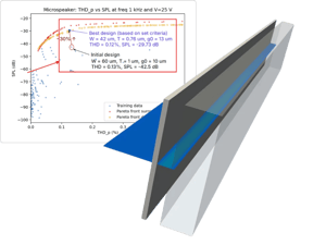
Predict multiphysics performance in milliseconds by training a validated statistical stand-in for the full solver.
Why surrogate models?

Explore design spaces that are too large to simulate point by point.

Get a performance prediction in milliseconds instead of minutes or hours.

Run the optimization, sensitivity, and yield studies that need thousands of evaluations.

Keep the full solver where it belongs: generating training data and validating the final design.
1. Sample the design space
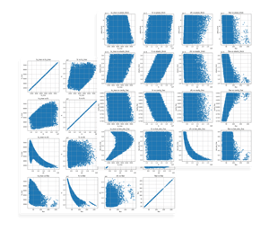
Choose the design variables and sample them with a space-filling design such as a Latin hypercube. A uniform grid wastes solves on regions where nothing interesting happens.
2. Generate the training data in parallel
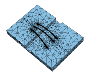
Run the sampled variants as concurrent sweeps in Quanscient Allsolve. Geometry and mesh regenerate automatically for every parameter combination, and the whole campaign can be scripted through the Allsolve SDK.
3. Fit the surrogate
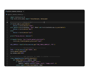
Train a model that maps design parameters to the simulated response — a Gaussian process when the dataset is small and smooth, a neural network when it is large or high-dimensional.
4. Validate, then exploit
Check predictions against held-out simulations the model has never seen. Once the error is acceptable, use the surrogate for optimization, sensitivity analysis, or Monte Carlo yield studies.
Ultrasound transducer
Designing a PMUT means trading sensitivity against bandwidth. 10,000 parallel simulations trained a surrogate that predicts both in under a millisecond, exposing the full Pareto front and a design with roughly double the fractional bandwidth. Open the white paper →

1. Dataset in minutes
10,000 Allsolve runs varying four geometric parameters, across four KPIs.
View full-size
2. Millisecond screening
The trained surrogate predicts performance in under 1 ms with roughly 1% error.

3. Pareto front, visible
The full sensitivity–bandwidth trade-off computed in seconds, constrained to the 12 MHz target frequency.

4. Verified improvement
Allsolve confirmed fractional bandwidth from 65% to about 100%, with +6.5% sensitivity.
View full-sizeMEMS microspeaker
Driving a microspeaker harder raises volume but also distortion. A nonlinear harmonic balance dataset of 12,500 simulations trained a surrogate that mapped the SPL–THD trade-off and then predicted manufacturing yield from the same model. Open the white paper -->

1. Nonlinear dataset in 20 minutes
Allsolve generated 12,500 nonlinear harmonic balance simulations in less than 20 minutes.
View full-size
2. Train the what-if engine/h5>That dataset became an instant performance predictor for new design ideas.
View full-size

3. Best trade-offs surfaced
A Pareto-optimal design with about 30% higher SPL while keeping THD below 0.15%, against a 1% target.

4. Yield from the same model
10,000 virtual prototypes under ±10% geometric variation predicted 72% manufacturing yield.
Piezoelectric material characterization
Identifying the full material matrices of a piezoelectric sample from measured impedance is a notoriously difficult inverse problem. Here the surrogate was trained to run backwards — from measured response to material properties.

1. Randomized dataset
10,000 simulations of a bulk PZT disc, randomizing stiffness, coupling, permittivity, and geometry for each run.

2. Inverse training
A model trained to take the simulation outputs, impedance magnitude and phase, and predict the material property inputs.
3. Instant characterization
Feed in a complex impedance spectrum, get the correct material properties back in milliseconds.
4. Quantified accuracy
Validation predicted the difficult-to-determine material matrices with error rates significantly below 5%.
View full-sizePatch antenna
A microstrip patch antenna was designed and tolerance-checked using 42 full-wave simulations, where a direct sweep of the same design space would have needed roughly 30,000. Open the article →
1. Space-filling start
30 Latin-hypercube designs run concurrently to fit the first Gaussian process, with no prior assumption about where the optimum sits.
View full-size
2. Infill on the ridge
The surrogate exposed a narrow resonance ridge, and later solves were concentrated along it rather than spread across the box.
View full-size
3. Solver certifies the candidate
The optimum was read off the fitted surface at W = 46.47 mm, L = 40.95 mm, then verified by full-wave sweep at 2.36 GHz with S11 = −36.8 dB.
View full-size
4. Same model, yield answer
Reused for Monte Carlo: 93% yield at S11 < −20 dB under ±0.15 mm etching, where 99% yield would need ±0.09 mm.
View full-sizeBond-wire radiation
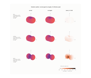
A six-parameter bond-wire geometry was sampled across 160 designs and five frequencies, a Gaussian-process surrogate was trained on the resulting 800 full-wave solves, and the fitted model now reconstructs a complete 3D radiation pattern in milliseconds. Open the article →
1. Parametric geometry, meshed automatically
Six geometry parameters plus frequency, with geometry and mesh regenerated for every combination. Typical models run 0.7–1.4 million DoF.
View full-size
2. 800 solves in 81 minutes
160 Latin-hypercube geometries at five frequencies each, submitted as 16 concurrent sweeps, with reported passivity of 0.9998–1.0000.
View full-size
3. Compress, then fit
Each pattern was reduced from 4,376 sampled directions to 25 spherical-harmonic coefficients before Gaussian processes were fitted to them.
View full-size
4. Validated on held-out designs
Across 32 designs never seen in training, the median RMS error over the main beam was 0.350 dB, and a full 3D pattern now takes about 1.5 ms to rebuild.
View full-sizeThe simulation platform behind the surrogate
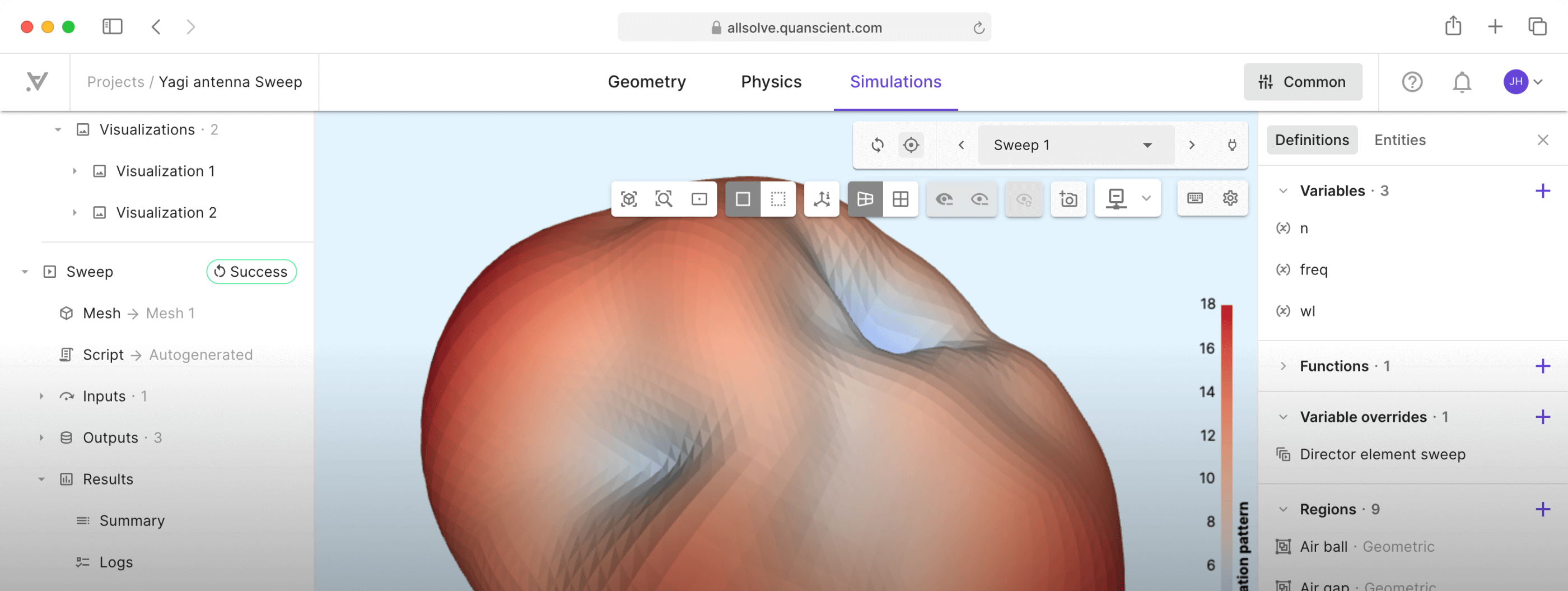

Training data in parallel
Hundreds or thousands of variants run concurrently, so a dataset takes minutes of elapsed time rather than days.

Natively coupled multiphysics
Train surrogates on genuinely coupled responses — electromagnetic, structural, acoustic, thermal — not on one physics at a time.

Scriptable campaigns
The Allsolve SDK samples the design space, creates parameter overrides, runs variants, and collects results, so a campaign is reproducible and extendable.

Validation on demand
High-fidelity solves stay one call away, for held-out testing and for certifying the final candidate.
MultiphysicsAI is this method, productized: managed training, physics-aware neural networks, and design-space visualization. Learn about MultiphysicsAI →
Real-world examples
Ultrasonic transducer
A dataset was generated, a fast model revealed the best trade-offs, and Allsolve verified designs with higher bandwidth and sensitivity.

1. Dataset in hours
~10,000 Allsolve runs across geometry variants and four KPIs.


Ultrasonic transducer
A dataset was generated, a fast model revealed the best trade-offs, and Allsolve verified designs with higher bandwidth and sensitivity.
1. Dataset in hours
~10,000 Allsolve runs across geometry variants and four KPIs.
Ultrasonic transducer
A dataset was generated, a fast model revealed the best trade-offs, and Allsolve verified designs with higher bandwidth and sensitivity.
1. Dataset in hours
~10,000 Allsolve runs across geometry variants and four KPIs.

How could physics-aware AI benefit you?
Get in touch now to discover the opportunities MultiphysicsAI could open for your work.
Case examples and other resources
White paper
Quanscient MultiphysicsAI for PMUT design
See the full step-by-step example of improving ultrasound transducer design with Quanscient MultiphysicsAI.
Open white paper →
White paper
Quanscient MultiphysicsAI for MEMS microspeaker design and optimization
A full breakdown of a MEMS microspeaker case with AI-driven design exploration.
Open white paper→

White paper
Accelerating engineering design with neural surrogates
Learn the 5 key stages for accelerating engineering work with neural surrogates.
Open the white paper→