Designing a patch antenna with a surrogate model

Key takeaways

• Using a baseline two-variable patch antenna for clear visualization, this example demonstrates a scalable, surrogate-based workflow designed to replace brute-force sweeps in complex engineering problems.

• The workflow efficiently combines Latin hypercube sampling, a Gaussian-process surrogate, and targeted infill, reserving the expensive high-fidelity FEM solver strictly for final validation.

• Using just 42 usable simulations, the surrogate successfully resolves the narrow 2.36 GHz resonance ridge, proposes W = 46.47 mm and L = 40.95 mm, and the full-wave check verifies an S11 of −36.8 dB.

• The exact same surrogate is then reused for a near-instant Monte Carlo yield analysis, showing 93% yield at S11 < −20 dB for standard ±0.15 mm etching and establishing a ±0.09 mm tolerance requirement for 99% yield.

Introduction

Antenna optimization is often framed as a geometry problem: vary a few dimensions, simulate each candidate, and choose the best result. That approach is straightforward when each simulation runs quickly and the design space is small. It becomes much less practical when each point requires a large 3D full-wave solve.

This example considers a rectangular microstrip patch antenna on a substrate with relative permittivity εr = 2.2 and thickness h = 1.57 mm. The design variables are patch length and width. Everything else, including the feed, transformer width, substrate, and board size, is held fixed. The objective is to place the resonance at 2.36 GHz, obtain a strong impedance match, and then understand how sensitive that design is to manufacturing variation.

While optimizing a two-variable patch antenna is a standard introductory problem, it serves as an ideal illustrative example. By keeping the geometry simple and restricting the design space to just length and width, we can clearly visualize how the surrogate model behaves (like the resonance ridge) without getting bogged down in the complexities of a multi-parameter design. The methodology demonstrated here, however, seamlessly scales to highly complex, high-dimensional engineering problems.

The workflow uses high-fidelity finite-element simulations to generate a limited set of training data, fits a Gaussian-process surrogate, uses that surrogate to select additional simulations, and finally validates the selected design again with the full solver. The surrogate is then reused for a manufacturing-yield study.

The design problem

36–46 mm for length and 25–55 mm for width. The performance quantity is S11, the reflection coefficient. Lower S11 means less incident power is reflected back toward the source.

As a rule of thumb, −10 dB corresponds to about 90% of incident power not being reflected, while −20 dB corresponds to about 99%. The target in this study is resonance at 2.36 GHz with as deep a match as practical.

Each design evaluation is a full 3D electromagnetic simulation with roughly 1.6 million degrees of freedom. The measured solve latency is about two minutes on a three-node machine. At 0.1 mm resolution, a direct sweep over the two-dimensional design box would require about 30,000 designs, corresponding to roughly 13 days at the measured throughput.

The practical budget is closer to 40 simulations. In this two-variable illustrative example, a direct sweep might still seem somewhat imaginable if you have enough time. However, if we were optimizing 5 or 10 parameters (like feed inset, substrate properties, and parasitic elements), a brute-force sweep becomes mathematically impossible. The surrogate-based workflow is designed exactly for those higher-dimensional realities, even though we use a two-parameter space here so you can easily see the results on a graph. Whether with 2 parameters or 10, the central question remains the same: not how to simulate every candidate, but how to choose a small number of simulations that reveal enough of the design space to make a defensible design decision.

Figure 1. Closed-loop workflow combining full-wave FEM with a surrogate model. The solver generates and validates data; the surrogate is used to explore the design space between those expensive solves.

What is a surrogate model?

A surrogate model is a cheap statistical stand-in for the expensive simulator: run a modest number of real simulations, fit a function through them, then predict anywhere in the design space in microseconds instead of minutes.

Here, the surrogate is a Gaussian process. It is smooth, needs very few samples, and returns an uncertainty estimate with every prediction. That uncertainty is what tells us where the next simulation is worth running.

The workflow

The workflow starts with a Latin hypercube sample of 30 designs: a space-filling spread over the whole box, with no prior assumption about where the answer is. The designs are simulated concurrently and used to fit the first Gaussian process.

Next comes infill: eight more designs are selected where the match is predicted deep or where the model is still uncertain. The Gaussian process is refit and the loop repeats. In total, the study uses 42 usable simulations and about 25 minutes of wall-clock time, with variants run concurrently.

This distinction matters. The first 30 points are intended to cover the whole box without assuming where the optimum lies. Later points are deliberately concentrated near the part of the design space that matters for resonance and matching.

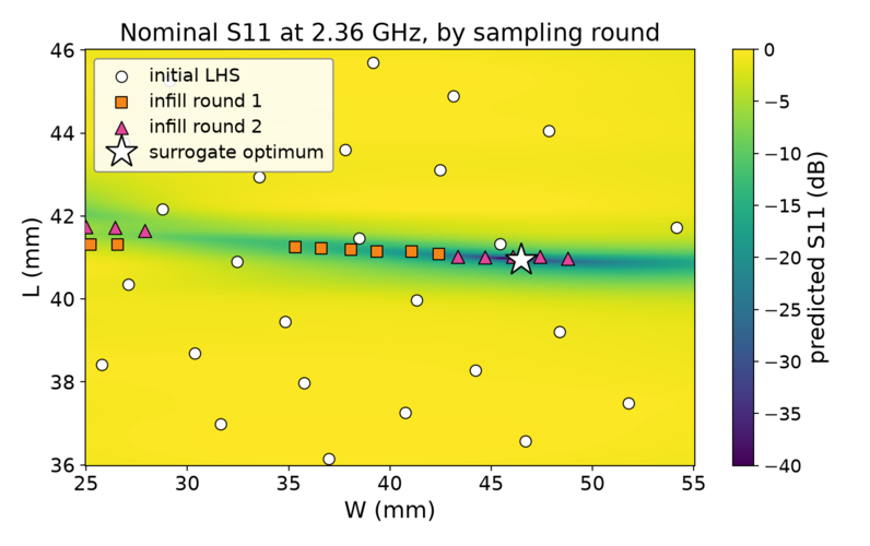
Figure 2. Predicted S11 at 2.36 GHz across patch width and length. White markers show the initial Latin-hypercube sample, while the later infill rounds concentrate along the narrow resonance ridge. Because we are using a simple two-variable example, we can visually plot the entire design space to understand exactly how the surrogate focuses on this ridge, a process that happens invisibly in higher-dimensional real-world problems.

Surrogate result

The surrogate shows a thin curved ridge in the width–length plane. Off that ridge, there is no resonance at 2.36 GHz. This is why a uniform brute-force sweep is inefficient: most of the design box does not contribute useful information about the resonance locus.

The infill rounds concentrate on this ridge. All 16 infill points sit on it, so each pass spends the expensive full-wave simulations where they matter most.

The reported optimum is not one of the simulated training points; it is read off the fitted surface. The candidate is then validated with the high-fidelity FEM solver. The surrogate proposes the design, and the full solver certifies it.

Result: the design

The selected geometry is W = 46.47 mm and L = 40.95 mm. The full-wave frequency sweep places the resonance at 2.36 GHz and gives S11 = −36.8 dB, which is well beyond the −20 dB criterion used later in the manufacturing analysis.

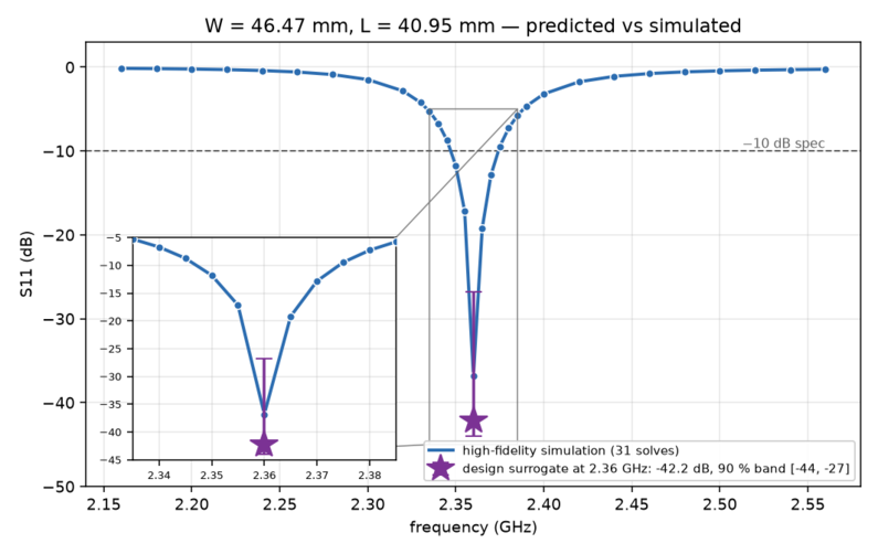
Figure 3. Frequency response of the selected design. The high-fidelity simulation verifies that the resonance occurs at 2.36 GHz and that the achieved S11 is substantially below the −20 dB criterion.

The important point is procedural: the surrogate narrows the search and proposes the geometry, while the final reported electromagnetic performance comes from the full solver.

Yield analysis

Once the surrogate is available, it can be reused to answer other engineering questions. Manufacturing yield is one example.

Assume the fabricated patch dimensions vary because of PCB etching. The presentation models this as ±0.15 mm at 3σ for both W and L. To estimate yield, the dimensions are perturbed repeatedly, the resulting S11 is evaluated, and the fraction of samples meeting a chosen specification is counted.

About 10,000 evaluations by simulation would take roughly four days per candidate design at the measured rate. The same 10,000 evaluations through the surrogate take less than one second.

For the selected design, the surrogate-based Monte Carlo study reports 100% yield for S11 < −10 dB and 93% yield for S11 < −20 dB.

Figure 4. Predicted probability of meeting S11 < −20 dB under ±0.15 mm etching variation. The high-yield region forms a narrow band in the width–length plane.

How tight must the process be?

The yield surface also makes it possible to reverse the question. Instead of asking how a given process tolerance affects yield, we can ask what tolerance is required to achieve a target yield.

Under the stated assumptions, standard ±0.15 mm etching gives 93% yield at the −20 dB requirement. Reaching 99% yield requires the process tolerance to tighten to approximately ±0.09 mm at 3σ.

That turns the electromagnetic model into a manufacturing requirement: the simulation campaign does not stop at identifying a nominal optimum, but connects the design to a quantitative fabrication tolerance.

Figure 5. Yield at the −20 dB criterion as a function of etching tolerance. The 99% target is reached at approximately ±0.09 mm, compared with 93% yield at the ±0.15 mm reference process.

What it cost

The workflow uses 42 high-fidelity simulations for training, completed in about 25 minutes of wall-clock time with concurrent execution. The yield study then evaluates the surrogate 2.74 million times.

The same questions asked directly by simulation are estimated at roughly 1,200 days. This comparison belongs to this specific design space, measured throughput, and yield study; it is not a generic speedup factor.

The method is most useful when each simulation is expensive, the design space is large enough that brute force is unattractive, and the engineering question involves exploration, optimization, or robustness rather than a single validation run.

Conclusion

This patch-antenna example shows a practical division of labor between a high-fidelity solver and a surrogate model. The solver is used where electromagnetic accuracy is required: to generate training data and to validate the final candidate. The surrogate is used where coverage matters: to interpolate between simulations, focus additional samples, and evaluate many manufacturing perturbations quickly.

With 42 usable full-wave simulations, the workflow identifies a design at W = 46.47 mm and L = 40.95 mm, verifies −36.8 dB S11 at 2.36 GHz, and then extends the same model to manufacturing yield. Under the stated ±0.15 mm etching assumption, the design reaches 93% yield at −20 dB; a 99% yield target implies a tighter tolerance of about ±0.09 mm.

The useful outcome is therefore not only a nominal antenna geometry. It is a validated design together with a quantitative view of how the manufacturing process affects whether that design will meet specification.

Ultimately, this baseline patch antenna serves as a clear, visualizable vehicle for a much larger point. The true takeaway isn't the specific dimensions of the antenna, but the workflow itself. By mastering this surrogate-assisted approach on a simple model, engineers can confidently apply the exact same methodology to highly complex, multivariable designs where brute-force simulation is no longer an option.