Introduction
Bond wires are small, but at millimeter-wave frequencies their geometry can have a measurable effect on electromagnetic behavior.
Changes in wire spacing, loop height, orientation, or pad-to-pad distance can alter both the amount of unwanted radiation and the direction in which that radiation is emitted. Understanding these effects is useful when defining layout rules, but exploring a multidimensional geometry space directly with full-wave simulation quickly becomes expensive.
In this example, Quanscient Allsolve is used to generate a full-wave simulation dataset for a parametric bond-wire model. A surrogate model is then trained to predict the complete 3D radiation pattern for previously unseen geometries.
The objective is not to replace electromagnetic simulation. The full-wave solver remains the source of training data and the reference used for validation. The surrogate provides a much cheaper way to explore the design space once that relationship has been sampled sufficiently.
The simulation problem
The model consists of a three-wire bond-wire array connecting a die pad to a PCB pad. The geometry is controlled by six design parameters: pad-to-pad span, loop height, spacing of the positive-side outer wire, spacing of the negative-side outer wire, yaw of the positive-side outer wire, and yaw of the negative-side outer wire. Frequency is included as an additional simulation input.
The two outer wires are parameterized independently, so the geometry does not need to remain symmetric. This makes it possible to study practical layout variations rather than restricting the model to an idealized symmetric configuration.
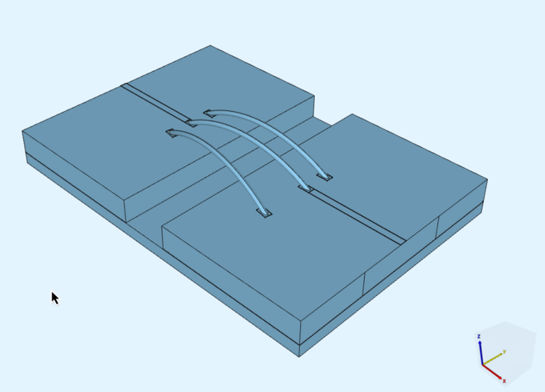
Figure 1. Parametric three-wire bond-wire geometry between the die and PCB pads. The outer wires can vary independently in spacing and yaw.
For each design, the geometry is regenerated and meshed automatically. A typical full-wave model contains approximately 700,000 to 1.4 million degrees of freedom. This automation is important because a parameter study is only practical if changing a geometry does not require manually rebuilding CAD and mesh definitions for every candidate.
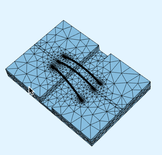
Figure 2. Example mesh generated for one geometry. Each parameter combination regenerates both the geometry and its mesh automatically.
Generating the training data
In this study, 160 geometries were sampled across the six-dimensional geometry space. Each geometry was evaluated at five frequencies, giving 800 full-wave training solves in total.
The variants were submitted as parallel sweeps rather than executed sequentially. Across 16 sweeps, the complete set of 800 solutions, including meshing, was generated in approximately 81 minutes. A typical sweep contained 50 variants and required about 1.5 minutes for meshing and 3.5 minutes for solving.
The reported passivity across the solves was 0.9998–1.0000. Parallelism does not reduce the electromagnetic work required for an individual design; it reduces the elapsed time required to generate a large dataset by running independent variants concurrently.
Quanscient Allsolve
High-throughput multiphysics simulation for RF
Run massive parametric sweeps and natively coupled multiphysics in the cloud with Quanscient Allsolve
Automating the campaign with Quanscient SDK
Running several hundred simulations manually would make this workflow difficult to reproduce and extend. The campaign was therefore controlled through the Allsolve SDK. A script defines parameter samples, creates geometry overrides, generates meshes, starts the simulations, and collects the resulting radiation-pattern data.
The six geometry parameters were sampled using a Latin hypercube and crossed with the selected frequency values. Multiple parameter combinations can be submitted together as one job, while completed variants can be collected even if another variant fails.
import allsolve
project = allsolve.Client().get_project_from_token()
# One override set: each parameter gets its list of values
sweep = project.create_variable_overrides(
"campaign",
[
("Xo", design.Xo),
("h", design.h),
("pitch_pos_y", design.pitch_pos_y),
("pitch_neg_y", design.pitch_neg_y),
("rot_posy_wire", design.rot_posy_wire),
("rot_negy_wire", design.rot_negy_wire),
("freq", design.freq),
],
)
# Mesh every variant, then solve them as one job
project.get_meshes()[0].create_override(sweep).run()
sim = next(
s for s in project.get_simulations()
if s.name == "Simulation 1"
)
sim.variable_overrides = sweep
sim.set_runtime(
allsolve.Runtime(
node_type=allsolve.CPU.CORES_4_64GB
)
)
sim.start()
while sim.is_running(refresh_delay_s=5):
pass
# Scalars for every variant, plus one pattern file each
PATTERN = "EM radiation pattern 3D"
data = sim.get_output_data(refresh=True)
for i in range(len(design)):
sim.save_output_field(
PATTERN,
output_dir=f"out/{i}",
sweep_index=i,
)
Figure 3. A programmatic campaign can sample the design space, create parameter overrides, run variants concurrently, and export one radiation-pattern result per design.
Using the same workflow for later batches also makes validation and dataset extension easier. New training points can be added without changing the underlying simulation model or rebuilding the campaign by hand.
Building the surrogate
Each full-wave simulation provides the radiation pattern for a given antenna geometry, sampled over thousands of directions. These simulation results are used to train Gaussian process models that learn how the radiation response varies with the design parameters.
The Gaussian processes use a Matérn 5/2 covariance function, with separate length scales for the input parameters and an independently estimated noise level for each predicted output. This allows the models to capture different sensitivities to the design variables while accounting for numerical variation in the simulation data.
Gaussian processes are a practical fit for this problem because the training set is relatively small: 160 geometries rather than tens of thousands of samples. They also return a predictive variance in addition to a mean, which becomes useful later when deciding where the design space needs more simulation data.
Once trained, the surrogate can predict the radiation pattern of a new geometry without requiring another full-wave simulation.
Testing the surrogate on unseen simulations
Training accuracy alone does not show whether a surrogate interpolates correctly. The model was therefore evaluated against 32 independently sampled held-out designs. Their frequencies were at least 1 GHz away from the training grid, and the surrogate predictions were saved before examining the corresponding full-wave results.
Across these validation cases, the median RMS error over the main beam was 0.350 dB. The 90th-percentile error was 0.970 dB, while the largest observed case was 1.277 dB.
Validation metrics:
Median / 90th percentile / worst
-
RMS error over main beam: 0.350 / 0.970 / 1.277 dB
-
Peak level: 0.088 / 0.202 / 0.245 dB
-
Peak direction: 1.56° / 4.55° / 10.80°
-
Total radiated power: 1.40% / 4.78% / 6.93%
-
Directivity: 1.10% / 2.21% / 4.50%
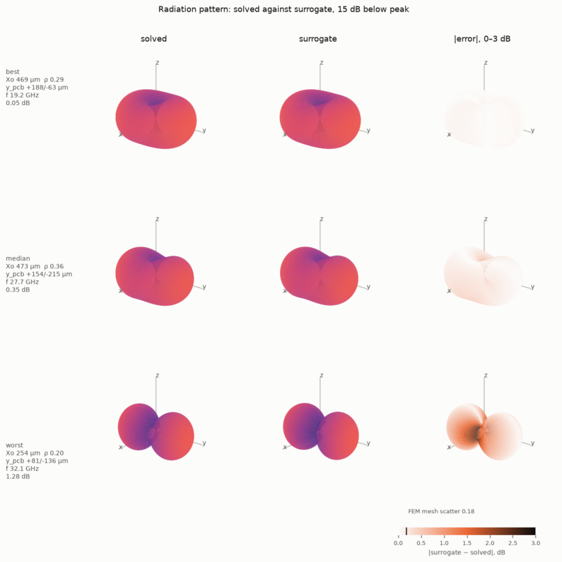
Figure 4. Full-wave and surrogate radiation patterns for representative validation cases. The error view shows the absolute difference between the two results.
The 3D comparison is useful because a single scalar metric can hide spatial differences. Principal-plane cuts provide a complementary view and make local disagreement around lobes or nulls easier to identify.
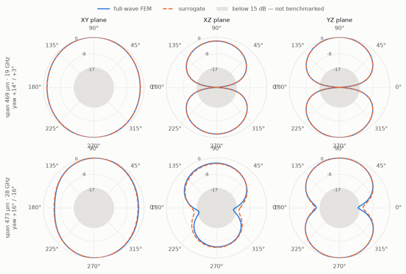
Figure 5. Full-wave FEM and surrogate predictions in the XY, XZ, and YZ planes for representative held-out geometries. Regions more than 15 dB below the peak are excluded from the benchmark.
For most of the main radiation pattern, the predicted and simulated curves closely overlap. The larger differences tend to occur near low-level regions and nulls, where a small absolute change in field magnitude can produce a larger difference in decibels.
Predicting uncertainity as well as the mean
A Gaussian process provides a predictive variance for each coefficient. By propagating the 25 coefficient variances through the spherical-harmonic representation, an uncertainty interval can be estimated for the radiation level at each direction.
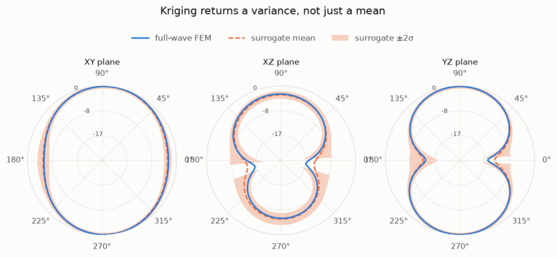
Figure 6. Full-wave result, surrogate mean, and predicted ±2σ interval in three principal planes.
Across all held-out designs and main-beam directions, 83% of the full-wave values fell within the predicted ±1σ interval, compared with a nominal 68.3%. At ±2σ, observed coverage was 95.5%, very close to the nominal 95.4%. For 26 of the 32 validation designs, the full-wave pattern stayed within the ±2σ interval at every main-beam direction.
Using uncertainty to choose new simulations
A surrogate is generally more reliable in well-sampled regions of the design space and less certain in sparsely covered regions. Candidate geometries can be evaluated with the surrogate before any additional full-wave solve is run, and higher predicted uncertainty can be used to prioritize the next batch of simulations.
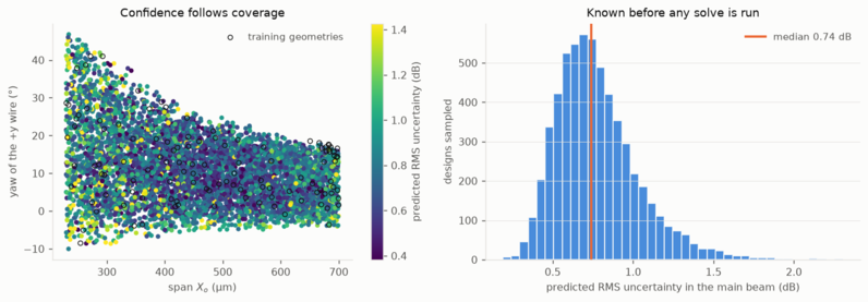
Figure 7. Predicted RMS uncertainty across candidate designs. Higher-uncertainty regions are natural candidates for additional full-wave sampling.
This gives a straightforward iterative workflow: simulate → fit → evaluate uncertainty → add samples → refit. Instead of increasing the training set uniformly, new solver time can be directed toward areas where the current model has the least support.
Simulation cost vs surrogate evaluation
The initial model required 800 full-wave training solves. With the simulations grouped into concurrent sweeps, the complete training dataset was generated in 81 minutes including meshing. Once trained, one surrogate evaluation that reconstructs a complete 3D radiation pattern takes approximately 1.5 ms.
The difference becomes important when the task changes from evaluating a few individual designs to scanning a large parameter space. A uniform five-level grid across the six geometry parameters plus frequency contains 5⁷ = 78,125 points. The source study estimates that solving this grid directly would take approximately 5.4 days under the same campaign setup.
Conclusion
This example combines three pieces rather than treating surrogate modeling as an isolated machine-learning task. First, the electromagnetic model is parameterized so that geometry changes can be generated and meshed automatically. Second, full-wave simulations are run concurrently to produce enough training and validation data within a practical elapsed time. Finally, the radiation pattern is compressed into a spherical-harmonic representation and interpolated using Gaussian processes that also provide prediction uncertainty.
For this dataset, the resulting surrogate reached a median main-beam RMS error of 0.350 dB on independently sampled validation designs, while evaluating a complete 3D pattern in approximately 1.5 ms.
The broader point is not that the surrogate removes the need for full-wave simulation. The simulations remain the source of the training data and the validation reference. The benefit is that, once the relationship between geometry, frequency, and radiation behavior has been sampled sufficiently, the fitted model can support rapid design-space exploration, sensitivity studies, and more targeted choices about which geometries to simulate next.