
From unit cell to the whole array
Elastic, acoustic and piezoelectric physics coupled across every element of a finite array — not one pillar at a time.
Array-scale • Coupled multiphysics • AI-driven optimization


“Quanscient Allsolve enables large-scale multiphysics simulations of PMUT and CMUT arrays that would be challenging to achieve with other simulation tools.”
 Nilavazhagan Subbiah, PhD
Staff Engineer, Infineon
“With Quanscient Allsolve, we were able to test different parameters to find the working design from the first iteration, saving three months in product development time.”
 Antony Hartley
CAE Consultant, IXI
Array-scale piezoelectric simulation, fully coupled
One model, all the physics, at array scale — carried from unit cell to finite array without rebuilding anything.

The whole finite array
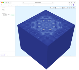
Absorbing PMLs replace the symmetry boundaries at the array edges. A 19×19-element array, about 9.1 million degrees of freedom, solves in under an hour on 112 cores.

Natively coupled physics
Elastic waves, acoustic waves and electrostatics with piezoelectric coupling, solved together in one transient run that covers the whole band.

Cloud scale, from code
The Python SDK builds and runs models through the API. Everything it creates is still an Allsolve project you can open and check.
Stack design in 39 seconds
The unit cell is still the right tool for the stack itself: under 19,000 degrees of freedom, 39 seconds a run — which is what makes it the model to run thousands of times. Watch the webinar →
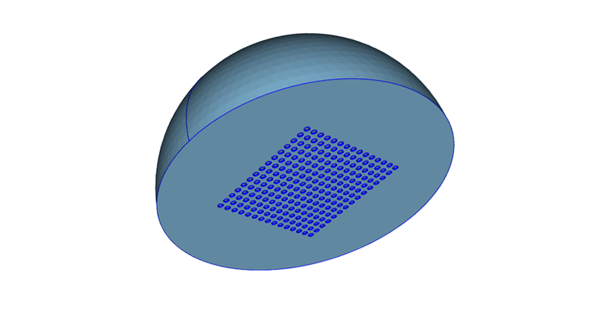
1. Define the stack once
Aptflex F30 backing, PZT-5H composite, hard-set matching layer and one wavelength of water at 1 MHz.
View full-size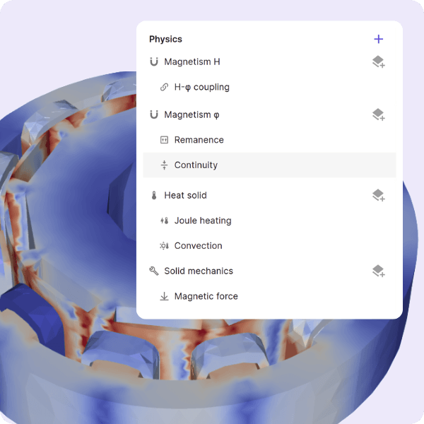
2. Four physics, one setup
Elastic waves, acoustic waves, electrostatics and the acoustic–structure interface, with PMLs top and bottom.
View full-size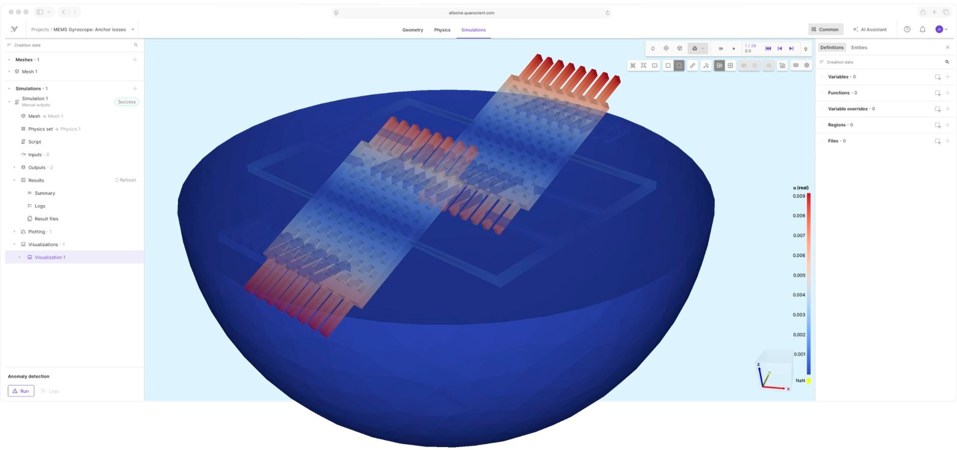
4. Every stack KPI from one run
The FFT gives centre frequency, −6 dB fractional bandwidth, resonance and coupling.
View full-sizeThe finite 19×19 array
Swap the symmetry boundaries for absorbing PMLs and the array becomes finite: 38×38 pillars, 19×19 elements, 9.1 million degrees of freedom. Watch the webinar →

1. Build the array, not the pillar
361 elements patterned from one parameterised definition, so element count and pitch stay variables.
View full-size
2. Parameterised, not hand-built
Pitch, kerf and element count are variables, so a different array size is a number rather than a rebuild.
View full-size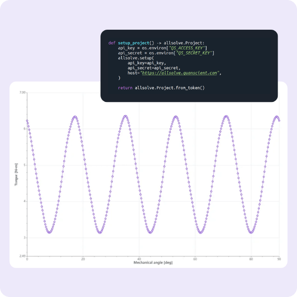
3. Drive one element
The central 2×2 pillars are driven and energy rings outwards: crosstalk, as it actually happens.
View full-sizeFar field without the water
A Kirchhoff integral gives the pressure anywhere outside the modelled domain, so beam patterns come out without meshing the water. Watch the webinar →

1. Place the points
An arc, spot, line or 2D grid, defined in the UI. Each green point is extrapolated to.
View full-size
2. On-axis pressure and the far-field beam
The pulse as it arrives at 50 mm, and the far-field beam taken along the arc.
View full-size
3. Results alongside everything else
Cartesian or polar in the browser, CSV for post-processing elsewhere.
A design question answered before manufacturing
A continuous epoxy matching layer couples every element to its neighbours. Sub-dicing it should widen the element beam — the question is what it costs. Watch the webinar →
1. Cut the matching layer
Diced along every element boundary and filled with silicone. Composite, backing and drive unchanged.
View full-size
2. Drive it and read the surface
The sub-diced array driven at its centre, with the displacement read straight off the aperture.
View full-size
3. A wider beam, and what it costs
The −6 dB beam width opens from 53.8° to 65.7°; peak Tx drops from 57.5 to 48.3 Pa/V.
View full-sizeAI-driven design space exploration
An optimizer is only as good as the numbers it optimizes, so the search layer proposes designs and Allsolve scores every one of them. Open the PDF summary →
1. The whole trade-off, visible
Grey dots are simulated designs, the red star the baseline, the purple line the Pareto front.
View full-size
2. Verified, not predicted
−6 dB fractional bandwidth from 69% to 84%, with higher peak sensitivity from the same stack.
View full-sizePiezoelectric material characterization
Identifying the full material matrices of a piezoelectric sample from measured impedance is a notoriously difficult inverse problem. Here the surrogate was trained to run backwards — from measured response to material properties.
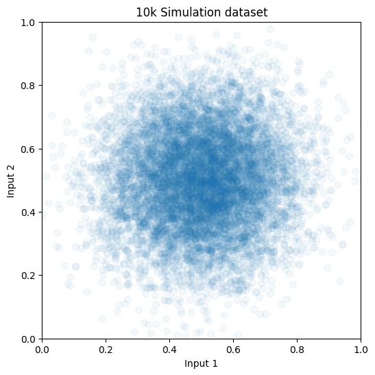
1. Randomized dataset
10,000 simulations of a bulk PZT disc, randomizing stiffness, coupling, permittivity, and geometry for each run.
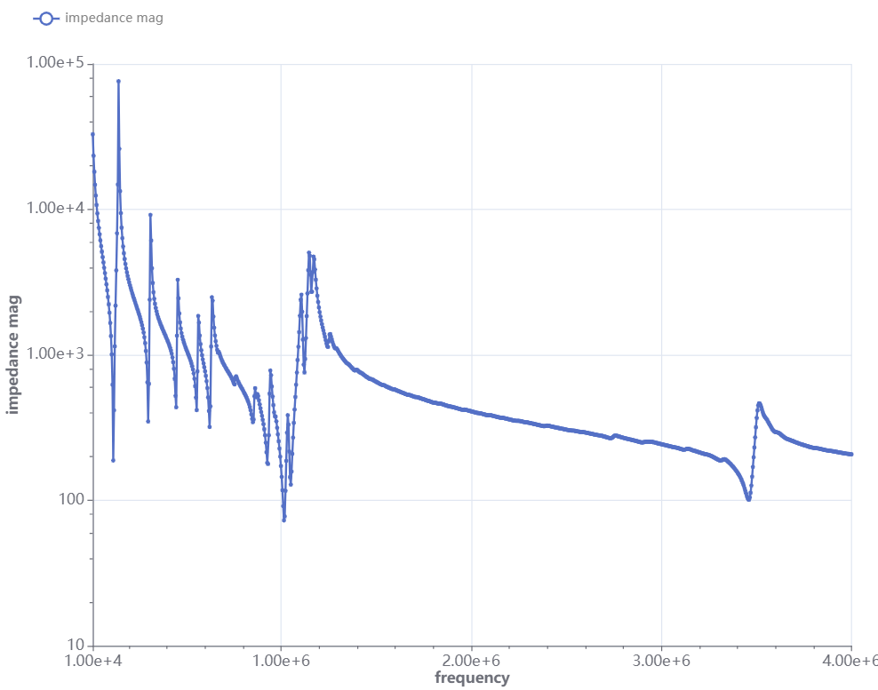
2. Inverse training
A model trained to take the simulation outputs, impedance magnitude and phase, and predict the material property inputs.
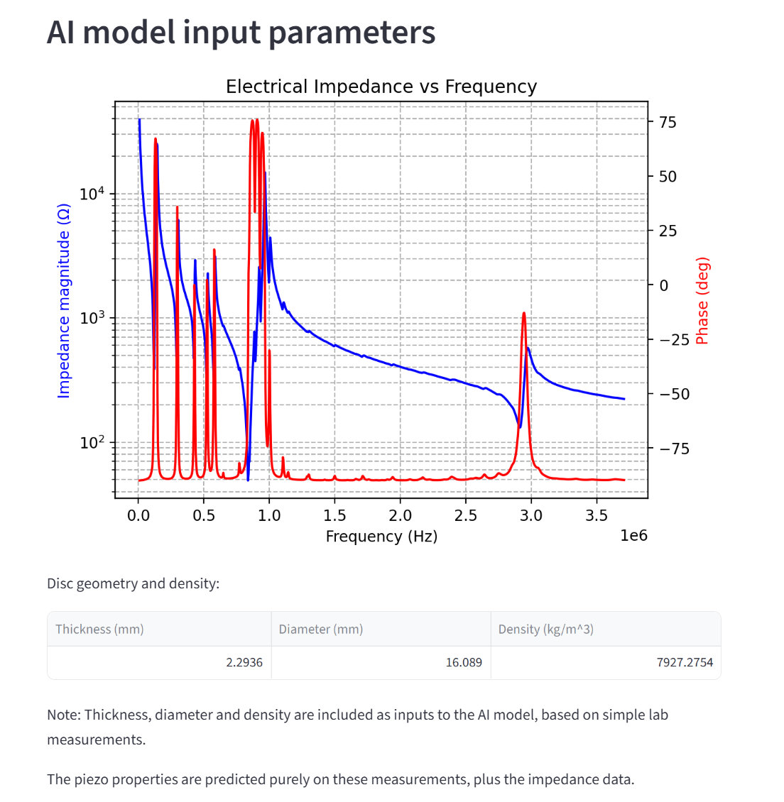
3. Instant characterization
Feed in a complex impedance spectrum, get the correct material properties back in milliseconds.
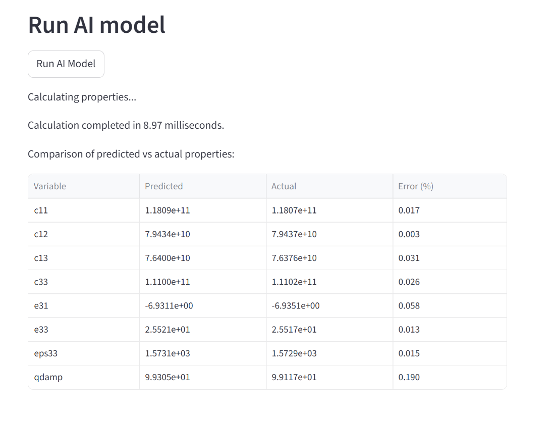
4. Quantified accuracy
Validation predicted the difficult-to-determine material matrices with error rates significantly below 5%.
View full-size
Not sure if Allsolve fits your transducer design?
Talk to our engineers about your application and how Allsolve could help in practice.
Case examples and other resources
Webinar + PDF summary
Simulating ultrasonic piezocomposite arrays
The unit cell, a 19×19-element array, acoustic extrapolation and a Pareto search, walked through live.
Download PDF summary →
White paper
MultiphysicsAI for ultrasound transducer design
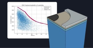
Thousands of simulations, a surrogate that predicts in milliseconds, and the trade-offs it exposes.
Open the white paper →
Case example
SAW filter design optimization
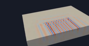
A 200-point frequency sweep in 90 seconds instead of 73 minutes, fully coupled.
Read the full article →
See how it could work for you
Submit the form to talk with our experts — we'll respond within one business day.
“Quanscient Allsolve's unique capabilities have helped us push the boundaries of what can be simulated in ultrasonic MEMS design.”
Nilavazhagan Subbiah, PhD — Staff Engineer, Infineon
Interested in just seeing an on-demand demo? Watch the 3-minute demo
Just want to know what it costs? See pricing and plans