Predicting nonlinear mode coupling in MEMS gyroscopes with full 3D harmonic balance

Introduction

Chances are there is a MEMS gyroscope in your pocket right now. These tiny sensors measure angular rate. In smartphones, they stabilize photos and video, track motion for games and augmented reality, and support navigation when satellite signals drop out. In cars, the yaw-rate sensor behind electronic stability control is a MEMS gyroscope, and electronic stability control is mandatory on new passenger cars in the EU and the US. Gyroscopes also stabilize drones and cameras and track head motion in VR headsets.

All vibratory MEMS gyroscopes work the same way. A silicon structure is kept vibrating in a drive mode. When the device rotates, the Coriolis force transfers part of that motion into a sense mode. The accuracy of the sensor therefore depends directly on how well its mechanical resonances behave.

This post describes a project with a MEMS gyroscope manufacturer: a full 3D simulation of nonlinear 1:2 mode coupling using harmonic balance in Quanscient Allsolve. The device and its results are confidential. To illustrate the physics, we use a closely related test structure published by Gobat et al. [1], of the same order of complexity as the device we simulated. We then explain what we did and what it took.

Why simulate before you fabricate?

Every MEMS design iteration means new masks, a new wafer run, packaging and testing. That takes weeks to months and costs a lot. Simulation moves this learning before fabrication. It predicts the drive and sense frequencies, the split between them, where spurious modes sit, and the quality factors. Most of this work relies on linear analysis. That is usually enough, since gyroscopes are designed to operate in their linear range. A linear analysis around the bias point even predicts how the DC bias shifts the frequencies. What it cannot predict is anything that depends on the vibration amplitude. Because gyroscopes have very high Q factors, even a small AC drive can produce vibrations large enough for that to matter.

When the physics turns nonlinear

The device

The structure in Figure 1 is representative of the device we simulated, and of the same order of complexity. It has four proof masses connected by folded springs to a central auxiliary component. It is made of polysilicon, measures 1.5 mm × 1.3 mm and is 24 µm thick. Electrodes on the substrate, 1.2 µm below the masses, handle out-of-plane actuation and readout [1]. Two modes matter here. The roll mode at 22,522 Hz is the one that gets driven. The spurious roll mode is at 43,386 Hz. Their ratio is 1.926, uncomfortably close to 2.

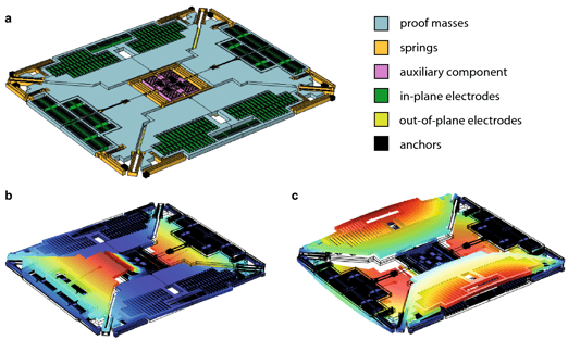
Figure 1. (a) The gyroscope test structure. (b) Roll mode, 22,522 Hz. (c) Spurious roll mode, 43,386 Hz. Reproduced from Gobat et al., Sci. Rep. 11, 16390 (2021) [1], CC BY 4.0.

The device operates at low pressure, so its quality factors are high: Q₁ = 2400 and Q₂ = 3480 [1]. As a result, the resonance peaks are only about 9 Hz wide. A nonlinear frequency shift of just 0.1% is enough to move the resonance by more than two peak widths.

Geometric nonlinearity

Linear analysis assumes small displacements. Once the slender suspension springs deflect far enough, their stiffness starts to depend on the deflection itself, for example because a bending beam also has to stretch. The resonance frequency then changes with amplitude, typically upward: the resonance hardens. The same nonlinear terms also couple modes, because deformation in one mode changes the stiffness seen by another.

Electrostatic softening from the DC bias

Gyroscopes are actuated and read out electrostatically, with a DC bias VDC plus an AC drive VAC. The electrostatic force grows as the gap closes, so the bias acts like a negative spring: the higher VDC, the lower the resonance frequency. This softening also depends on the vibration amplitude, and the bias pulls the structure statically toward the electrodes. Because the force depends on the deformed geometry, the electric field has to be solved on a geometry that moves with the structure.

The result: the resonance shifts and the peak bends

Together, these effects shift the resonance and bend the peak (Figure 2). Beyond a critical drive level, the peak folds over. Within a band of frequencies, two stable solutions then coexist, and the response jumps between them depending on the sweep direction.

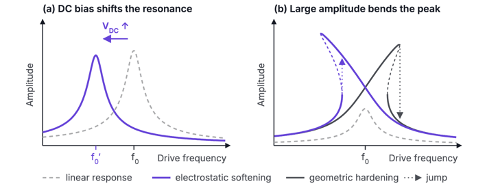
Figure 2. Schematic. (a) The DC bias lowers the resonance frequency. (b) At large amplitude, the peak bends right (hardening) or left (softening). Dashed segments are unstable, and dotted arrows show the jumps in an upward frequency sweep.

Figure 3 shows this on the test structure of Figure 1. As VDC rises from 4.145 V to 4.47 V, the roll resonance moves down by about 200 Hz, roughly twenty peak widths. The peaks also bend to the left and develop jumps. The inset shows the key detail. The roll frequency f1 falls faster than half the spurious roll frequency, f2/2, and the two cross near 4.3 V. The bias has tuned the frequency ratio to exactly 2.

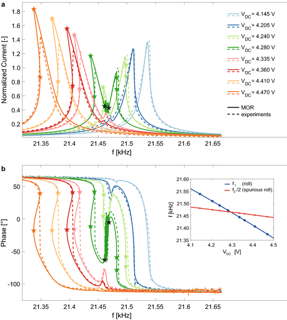
Figure 3. Roll-mode response for increasing V_DC at V_AC = 3.16 mV, model (solid) and experiment (dashed). Inset: f₁ and f₂/2 against V_DC. Reproduced from Gobat et al., Sci. Rep. 11, 16390 (2021) [1], CC BY 4.0.

Modal coupling: when two modes exchange energy

In a linear structure, modes are independent. Nonlinearity lets them exchange energy, and the exchange becomes strong when their frequencies sit near an integer ratio. This is called an internal resonance. In the 1:2 case, driving the lower mode produces, through the nonlinearity, a force at twice the drive frequency. That is exactly where the second mode resonates. It responds strongly, amplified by its high Q, and its motion in turn feeds energy back into the driven mode.

Figure 4 shows the result at VDC = 4.28 V. The single roll peak splits in two. In a narrow band between the peaks, the motion never settles into a periodic state. Instead it becomes quasi-periodic, and the measured signal fluctuates. The frequency ratio was 1.926 at zero bias. The bias brought it to 2, and the nonlinearities did the rest.

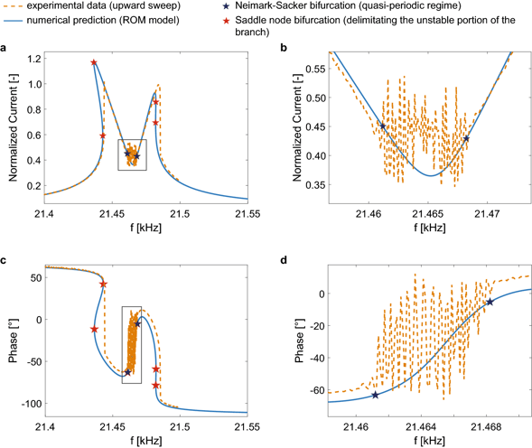
Figure 4. 1:2 internal resonance at V_DC = 4.28 V. The peak splits in two, with a quasi-periodic region in between (close-ups in b and d). Model in blue, experiment in orange. Reproduced from Gobat et al., Sci. Rep. 11, 16390 (2021) [1], CC BY 4.0.

1:2 is not the only dangerous ratio. Modes at 1:3 and other ratios can couple too, and a real gyroscope can have dozens of modes below five times its drive frequency.

Why it matters in a real gyroscope

A control loop holds the drive mode at a large, constant amplitude, because the Coriolis signal grows with drive velocity. Pushing the amplitude up can bring the device into the nonlinear regime:

• Frequencies move. Any drift in bias or amplitude becomes a drift in scale factor.

• Peaks bend and fold. Jumps and multiple stable states make the drive loop harder to control and cap the usable amplitude.

• Modes couple, and this is the most harmful effect. Energy leaks into a parasitic mode that is not part of the design. If that motion reaches the sense electrodes, or modulates the drive, the readout shows a signal even when the device is not rotating. This is a zero-rate output, or bias, error. In the quasi-periodic regime, the error also fluctuates over time.

Designers normally place parasitic modes well away from integer multiples of the drive frequency. The catch is manufacturing tolerances. Spring widths, layer thickness and electrode gaps all vary, and each mode depends on them in its own way, so the frequency ratio varies from device to device. A design whose nominal ratio is safely away from 2 can land on it for part of a production lot. The DC bias, as Figure 3 shows, can then pull the ratio exactly onto 2.

How it is simulated today: lumped reduced-order models

Simulating the full 3D nonlinear dynamics is generally considered too expensive. The standard tool is therefore a lumped, or reduced-order, model. The motion is reduced to a few modal coordinates, here the roll and spurious roll modes. Each one behaves as an oscillator with its own frequency and Q factor, and the oscillators are coupled by nonlinear mechanical and electrostatic forces. The resulting handful of equations can be solved in seconds.

The model coefficients come from simplified theories, from fits to measurements, or from FEM. Gobat et al. extract theirs from a series of static nonlinear FEM analyses and from electrostatic computations of the deformed structure. They fit the results with third-order polynomials and take the Q factors from a separate damping model. Their model matches the experiments in Figures 3 and 4 very well without any calibration, which makes it a state-of-the-art lumped model.

The limits of lumped models

Lumped models are only as predictive as the assumptions built into them:

• You must know in advance which modes couple. The paper notes that methods built on linear modes "must also include all the coupled high-frequency modes that are often difficult to identify" [1]. A roll/spurious-roll model can only predict 1:2 coupling between those two modes.

• Many models need hardware first. Their coefficients are in most cases "obtained from simplified electro-structural theories" or "calibrated on experimental data" [1].

• Approximations are built in. They include moderate deformations, a quasi-static treatment of all other modes, polynomial fits over a prescribed amplitude range, and quasi-static electrostatics.

• The drive is linearized. Assuming the AC drive is much smaller than the DC bias drops the part of the electrostatic force at twice the drive frequency. That is exactly where the 1:2 partner mode resonates.

• Damping is an input, not a result, and every design variant means repeating the extraction.

The paper also explains why the full model is avoided. With electromechanical coupling it has about 17 million degrees of freedom, and the authors estimate that a time-domain analysis would take about one year on a 16-core workstation. They describe harmonic balance on the full model as "overwhelmingly complex and time consuming" [1]. That is the gap this project set out to close.

Harmonic balance: solving for the steady state directly

A gyroscope driven at fixed voltages and a fixed frequency settles into a periodic steady state. Harmonic balance computes that state directly. It writes every field as a truncated Fourier series in time: a constant term plus sine and cosine terms at multiples of the drive frequency ω.

The same expansion is applied to the electric potential and to the mesh deformation in the gaps. The unknowns become 2N + 1 spatial fields, each a full 3D finite element field. Requiring each harmonic to balance gives one large nonlinear system, solved with Newton iterations. The truncation order N sets what the solution can capture:

• k = 0: the static deflection caused by the DC bias.

• k = 1: the response at the drive frequency.

• k = 2: the 1:2 partner mode, driven both by the nonlinearities and by the electrostatic drive itself.

• k = 3 to 5: higher-order effects and couplings to modes near 3ω, 4ω and 5ω.

Why not a transient simulation?

Because of the Q factor. With Q in the thousands, a transient takes thousands of oscillation cycles to die out: about 5,000 to 8,000 cycles to settle to 0.1% here. Each cycle needs tens of time steps on a model with millions of unknowns, and all of that buys a single frequency point. No wonder [1] estimates about a year for a time-domain analysis. For high-Q resonators, time-domain analysis is not realistic, and harmonic balance, which skips the transient entirely, is essential.

What full 3D harmonic balance in Allsolve adds

• Geometric nonlinearity comes from fully nonlinear solid mechanics on the real geometry, with no polynomial fit and no prescribed amplitude range.

• Electrostatic softening comes from the 3D electric field on a mesh that deforms with the structure, under the full DC plus AC drive. The static pull and the force at twice the drive frequency are both included.

• Modal coupling emerges from the solution itself. No modes are chosen in advance, so any mode near 2ω to 5ω shows up.

Mechanics, electrostatics and mesh deformation are solved in a single strongly coupled system on the full 3D geometry. Every effect the finite element model can represent is therefore accounted for, not just the ones chosen in advance. For example, the electrostatic force automatically includes the fringing fields at electrode edges and between comb fingers, instead of relying on an idealized parallel-plate formula. The nonlinear response follows from geometry, materials and voltages alone.

Why harmonic balance is rarely used for this

The compute cost. The number of unknowns is multiplied by 2N + 1, so millions become tens of millions, and the Jacobian couples every harmonic to every other one. That is far beyond a workstation. Such problems need a solver that scales across many cores.

Availability. Harmonic balance is well established in RF circuit simulation, and it is commonly available for lumped MEMS models, which are typically solved in circuit-level and system-level simulators. The reduced-order model in [1] is itself solved with harmonic balance. The general form needed for the full 3D model is rarely available. It combines nonlinear solid mechanics, electrostatics and a deforming mesh, all expanded in harmonics and fully coupled.

What Quanscient Allsolve achieved

In this project, Allsolve ran full 3D harmonic balance simulations of a realistic gyroscope of the same order of complexity as the one in Figure 1. Nonlinear solid mechanics, electrostatics and mesh deformation were strongly coupled.

This is not a like-for-like comparison with the one-year estimate in [1], since the model, software and hardware all differ. It does show that the problem has gone from out of reach to minutes per frequency point. Allsolve can also run many frequency points in parallel in the cloud.

From 1:2 to 1:5 in a single run

All harmonics from 0 to N are solved together. A single run with N = 5 therefore resolves 1:2, 1:3, 1:4 and 1:5 couplings simultaneously, without choosing modes beforehand (Figure 5).

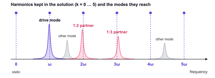
Figure 5. Schematic. Any structural mode close to a retained harmonic, such as a 1:2 or 1:3 partner of the drive mode, is captured automatically in the same solve.

Mapping the design space, however, takes many runs. Peaks are about 9 Hz wide but move by hundreds of hertz with bias, so each frequency response needs tens of frequency points. The coupling also depends on both VDC and VAC, and the crossing band is only a fraction of a volt wide. A dense grid of operating points fine enough to resolve it would need over ten thousand solves, or more than a hundred thousand core-hours for a single design.

Surrogate models: mapping the whole drive range

A surrogate model solves this problem. It is a cheap stand-in for the solver that predicts the full frequency response at any bias and drive level, together with a map of where the response stops being a clean resonance. The surrogate is built from full 3D harmonic balance results, and it predicts new operating points almost instantly.

Physics plus data

There are two classical ways to build a surrogate. A reduced-order model, like the lumped models above, is physically transparent. But it needs access to the solver's internals and a derivation for every device, and it gives no estimate of its own error. A black-box emulator, typically a Gaussian process, is a statistical model that interpolates between data points and reports its own uncertainty. It needs nothing but the solver's inputs and outputs. However, it doesn't know that a resonance has a peak that moves with bias, so it needs far more data to discover that.

Our surrogate takes a middle path. Its backbone is the smallest physics that produces the split: two coupled oscillators, one at the drive frequency and one at twice it. They are described by seven parameters, such as the two resonance frequencies, their widths and the coupling strength. These parameters are fitted to every solved frequency response. Each one then gets a Gaussian process over bias and drive, so the surrogate can predict the full curve at an operating point it has never seen. A final Gaussian process learns a smooth correction for whatever the two oscillators get wrong. Unlike a lumped model, the coupling is learned from the full 3D results instead of being derived, and the correction fixes the two-mode physics where it falls short. Trained on of the order of ten frequency responses, the surrogate reached a mean error below 2% on a similar number of held-out ones (Figure 6).

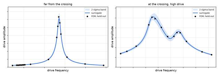
Figure 6. The surrogate against full 3D harmonic balance solves at two operating points it was never trained on: far from the crossing (left) and at the crossing at high drive (right). The shaded band is two standard deviations. Axis values are omitted because the device is confidential.

Uncertainty decides what to simulate next

Every prediction of the surrogate comes with an uncertainty band. The band is not decoration: it ran the campaign as an active-learning loop.

Figure 7 shows the campaign. From three clean curves, the surrogate already guessed the crossing bias. The two resonance frequencies can be measured on clean curves and extrapolated to where one is twice the other. What it did not know was the strength of the coupling, so its uncertainty was large there. Round one filled the corners of the domain, and round two went straight into the crossing. After two rounds, the unsafe zone is clearly delimited: a narrow band of bias, above a threshold drive level. We also checked the uncertainty band on several hundred solves the loop never used. It is slightly conservative and never overconfident, which is the right failure mode for a loop that relies on it.

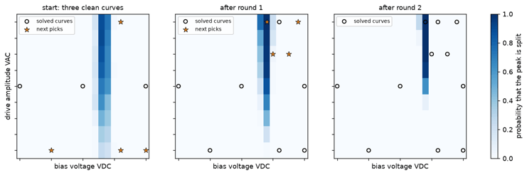
Figure 7. The campaign as the loop saw it, from the initial three curves through two rounds. Color is the surrogate's probability that the drive peak is split, over DC bias and AC drive amplitude. Circles are solved operating points and stars are the picks for the next round. Axis values are omitted because the device is confidential.

What it took

Each frequency point is an independent solve, and Allsolve runs all points of a sweep at the same time, each on its own set of cores. A sweep therefore takes of the order of ten minutes, however many points it has, and a full round of new operating points of the order of an hour. That turnaround is what makes the loop practical. With overnight queues, the same method would take weeks.

That is more than an order of magnitude fewer solves than a dense grid. Once trained, the surrogate explores the whole VDC–VAC range instantly. Building fast, physics-aware surrogates from Allsolve data is what Quanscient MultiphysicsAI is designed for.

Conclusion

In a MEMS gyroscope, the DC bias shifts the resonances and large amplitudes bend the peaks. When a parasitic mode sits near twice the drive frequency, the nonlinearities in the system can also couple it to the drive mode in a 1:2 internal resonance. The result is an output at zero rotation that factory trimming cannot reliably remove. Lumped models capture this when you already know which modes matter. They miss the modes you left out.

Full 3D harmonic balance in Quanscient Allsolve removes that blind spot. It solves all these effects in one strongly coupled run, with no transient to wait out. With a physics-informed surrogate driven by its own uncertainty, mapping the unsafe zone across the full drive range took of the order of 100 solves and of the order of an hour of wall-clock time. Mode-coupling risk can now be assessed before tape-out, instead of being discovered on the first wafer.

References

1. G. Gobat, V. Zega, P. Fedeli, L. Guerinoni, C. Touzé and A. Frangi, "Reduced order modelling and experimental validation of a MEMS gyroscope test-structure exhibiting 1:2 internal resonance," Scientific Reports 11, 16390 (2021). doi:10.1038/s41598-021-95793-y

Figures 1, 3 and 4 are reproduced without modification from [1] under the Creative Commons Attribution 4.0 International License. Figures 2 and 5 are schematic illustrations by Quanscient. Figures 6 and 7 show project results, with axis values omitted for confidentiality.