
Expert contributors for this post
Dr. Alexandre Halbach
CTO, Co-founder
Dr. -Ing. Abhishek Deshmukh
Team Lead - Application Engineering
Introduction
Nonlinear systems are everywhere in engineering, from how materials bend and stretch to how electrical circuits work. These systems don’t follow simple rules, which makes them challenging to analyze. Traditional approaches like transient simulation are often used to understand and characterize the system behavior, but these approaches have significant drawbacks. For one, they take a long time to simulate and often require manual fine-tuning to reach steady solutions (see Fig.1). Even after all that effort, the results can be noisy and difficult to interpret, especially when trying to extract frequency data.
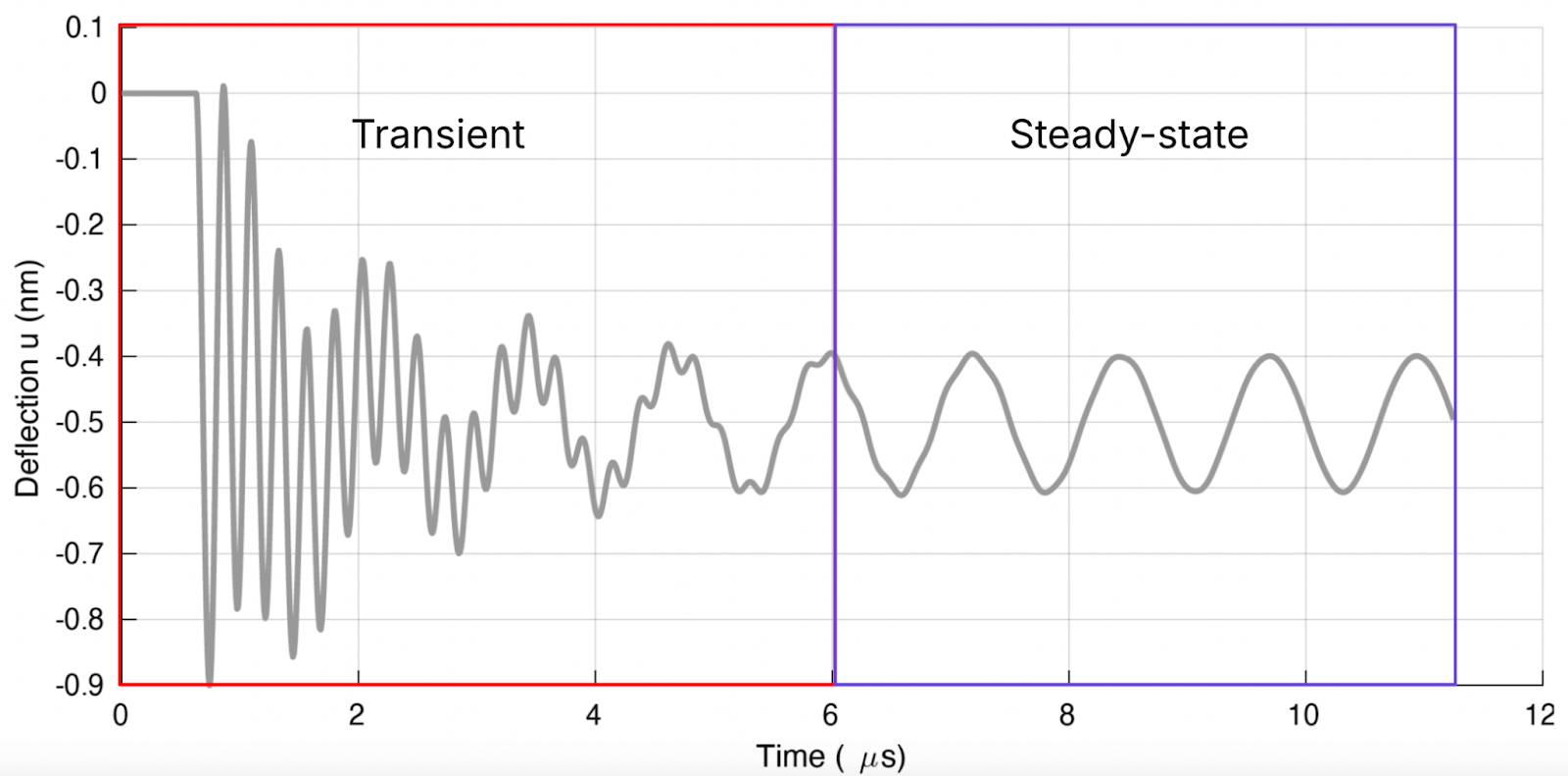
Fig. 1: Displacement over time showing transient behavior before reaching a steady periodic state [1].
A better approach is the harmonic balance method, which works directly in the frequency domain. This method doesn’t just look at the basic periodic pattern (or fundamental harmonic); it also captures the more complex patterns (higher harmonics) that come from the system’s nonlinear behavior. By doing so, it gives a complete picture of how the system behaves in frequency domain, making it an invaluable tool for engineers dealing with complex problems.
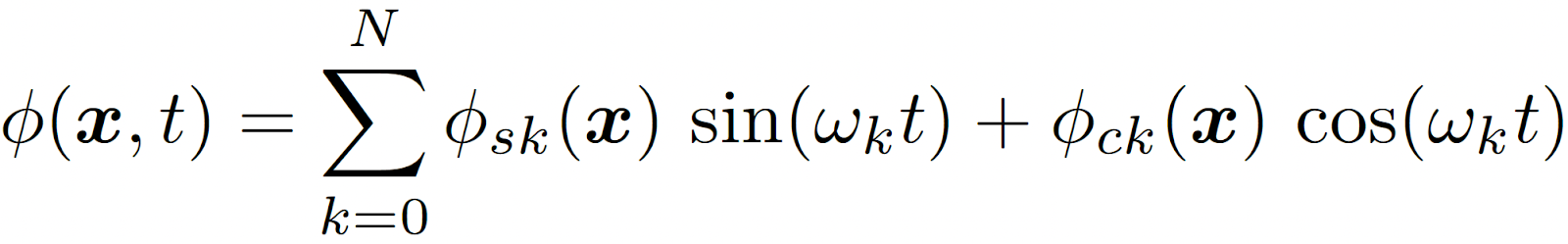
The harmonic balance method decomposes fields into a truncated Fourier series, which represents the system's behavior as a sum of harmonics, as shown in equation 1. These harmonics include not only those from the driving force but also new ones that emerge due to the nonlinearity of the system. This principle ensures that the method can accurately capture steady-state periodic behaviors even in highly complex systems.
By focusing on dominant harmonics, the method avoids unnecessary calculations, making it more efficient than transient simulations. This approach allows engineers to analyze nonlinear systems with precision and clarity, which is particularly useful for applications requiring detailed insights.
Eq. 1
Impact of Quanscient Allsolve's harmonic balance method in engineering
Harmonic balance has been a valuable method since its development in the 1970s [2], initially applied to simpler lumped models due to their lower computational costs. However, its application to the finite element method (FEM) has been historically limited by the rapid increase in computational demands and memory requirements as the number of degrees of freedom (DoFs) and harmonics grow. FEM models are inherently complex, involving a large number of DoFs that significantly escalate computational costs, especially when higher harmonics are included.
Quanscient Allsolve addresses these limitations by combining the harmonic balance method with the scalability of cloud computing. By leveraging on-demand cloud resources, Quanscient Allsolve eliminates the hardware bottlenecks of memory and processing power, enabling efficient application of harmonic balance to large-scale FEM models for nonlinear engineering problems in the frequency domain. It not only makes it possible to simulate systems previously considered too computationally intensive but also allows engineers to selectively analyze higher harmonics without simulating intermediate ones, thereby saving time and reducing unnecessary computations.
To date, no other commercial tools offer harmonic balance for FEM, particularly for multiphysics applications. Quanscient Allsolve distinguishes itself as the only tool providing this capability, offering engineers a novel and efficient approach to complex simulations.
Quanscient Allsolve
Scalable multiphysics simulations for MEMS design
See how Quanscient Allsolve expands MEMS design possibilities →
Case examples
AC Joule Heating [3]
Electrical systems, from the wiring in our homes to the circuits in our smartphones, generate heat as electricity flows through their conductors. This phenomenon, known as Joule heating, can significantly impact the performance and lifespan of these systems.
Simulations are used to predict and analyze Joule heating effects. By simulating different geometries, materials, and current loads, efficiency can be optimized in wire designs. This is especially important in applications with high currents or limited space, such as electronic devices and power transmission systems.
Simulation objective
A simple example for the demonstration of the key principle of the harmonic balance method.
The model- Aluminium filament with rectangular cross section (0.1 mm x 0.1 mm) and length of 1 mm
- Physics: Current flow + Heat solid
- Coupling: Joule heating
- Driven on one end by a sinusoidal current at a chosen fundamental frequency (f0) with the other end grounded
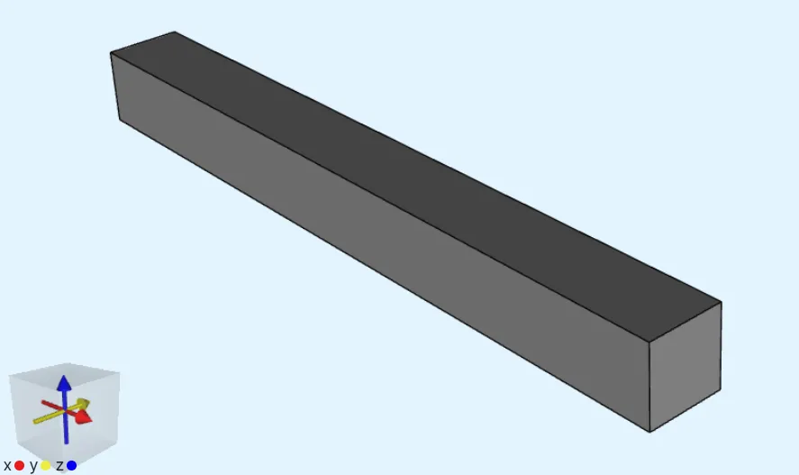
Fig. 2: Model view of the aluminium filament in Quanscient Allsolve.
Key results
Fig. 3: Temperature in transient simulations at f0 = 100 Hz and 400 Hz.
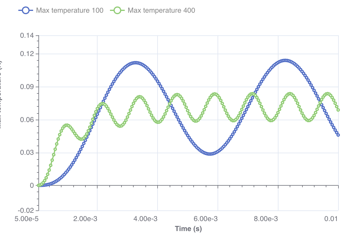
- Plots in Fig. 3 show the evolution of temperature for the current flow through the filament at fundamental frequency f0 = 100 and 400 Hz.
- Maximum temperature plot at steady state has a constant component and a periodically fluctuating component at a frequency twice that of fundamental frequency (2 x f0).
- These components can be captured with the harmonic balance method in the frequency domain as shown in Fig. 4. T1 is the constant component at zero frequency, T2 the sinusoidal part and T3 the cosinusoidal part at the fundamental frequency, and T4 the sinusoidal part and T5 the cosinusoidal part at twice the fundamental frequency.
- Joule heating is proportional to the square of applied current (I²). The sinusoidal applied alternating current at a fundamental frequency results in the constant heating of the filament with fluctuations about the constant temperature.
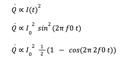
The temperature is governed by the diffusion equation.
The transient term above adds damping to the system with the temperature field, resulting in both sinusoidal and cosinusoidal components.
![]()
As clearly visible, in addition to the constant component, the rest of the contributions come from the second harmonic coefficients at frequency 2 x f0, and the fundamental harmonics (at f0) are zero.
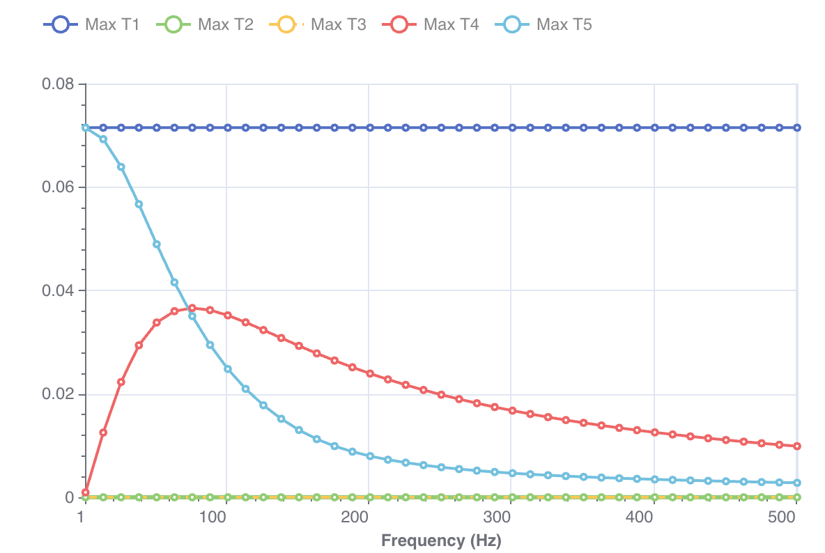
Fig. 4: Harmonic components of temperature in harmonic balance simulations at f0 between 1 Hz to 501 Hz in 41 steps
Key benefits demonstrated
The transient simulation approach was compared with the harmonic balance method and the key principles of the harmonic balance approach were clearly demonstrated.
Backbone curves [4]
Beams are fundamental structural elements used in a wide range of applications, from bridges and aircraft to microelectronics. However, beams are susceptible to vibrations, which can lead to fatigue, instability, and potential failure. Therefore, understanding beam vibration behavior is essential for engineers across various disciplines.
Simulation objective
Demonstration of the capability of the harmonic balance in capturing nonlinear behavior of the clamped-clamped beam.
The model
- A beam with rectangular cross section (0.03 m x 0.03 m) and length of 1 m
- Physics: Solid mechanics + Mesh deformation
- Coupling: Large displacements (Geometric nonlinearity)
- Driven by a sinusoidal load at a chosen fundamental frequency (f0)
Key results
Mechanical resonance is represented by maximum displacement versus driving frequency
Fig. 5 shows the maximum displacement over frequency without geometric nonlinearity. The linear behavior shows the resonance peak.
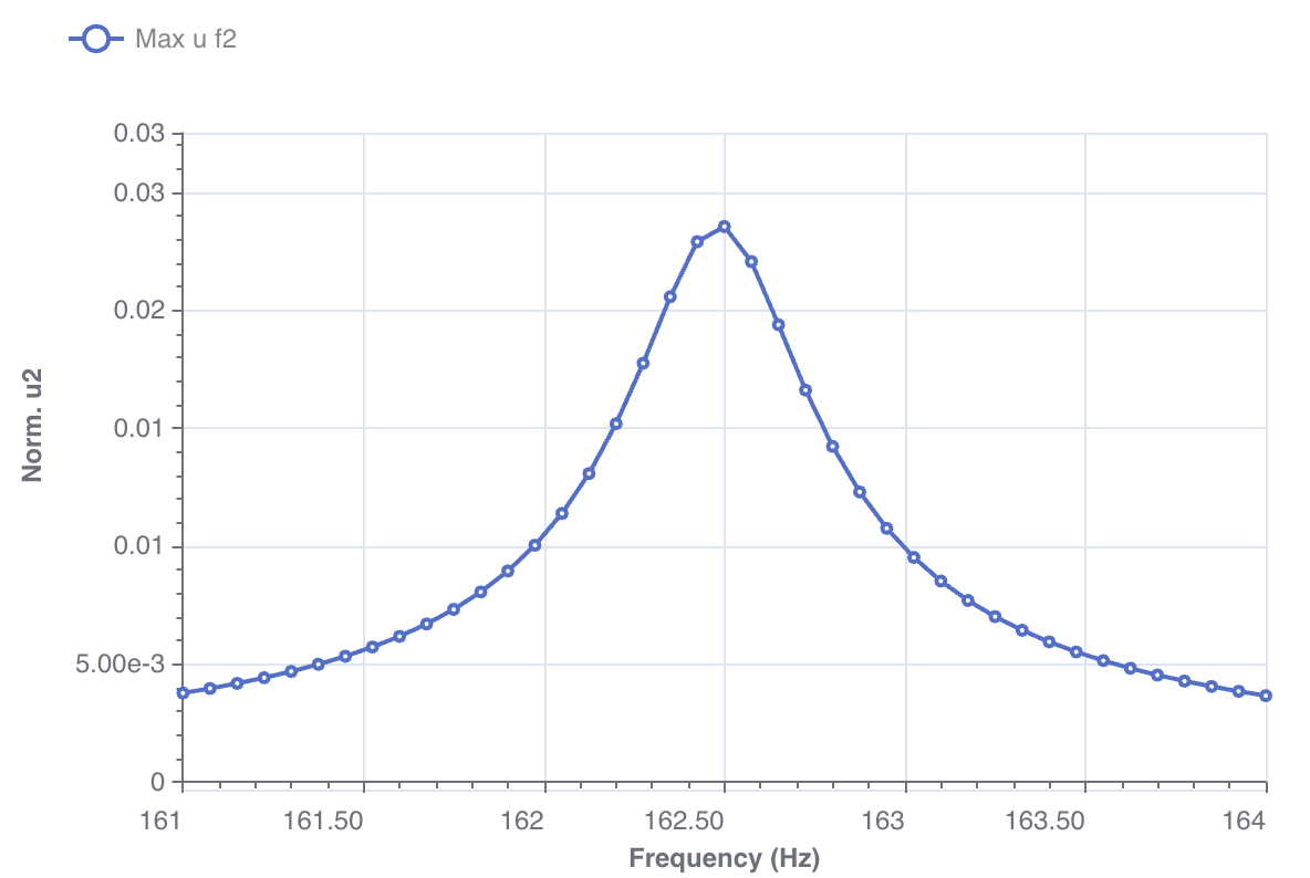
Fig. 5: Maximum displacement vs. frequency sweep without geometric nonlinearity.
Considering geometric nonlinearity, multiple valid solutions exist at a chosen driving frequency as evident from literature [5] (see Fig. 6), which makes transient simulations difficult in this case as clearly shown by the backbone-shaped curve.
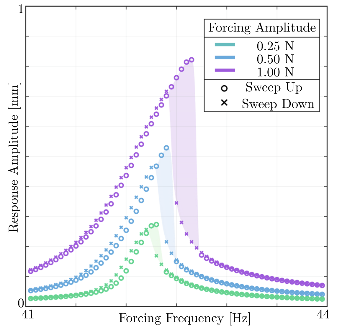
Fig. 6: Experimental data from Hayashi et al. [5].
However, Quanscient Allsolve can trace the points on each branch using the harmonic balance approach (see Fig. 7). Note that the simulation setup in this example different from that of Hayashi et al. [5] and hence not comparable and not intended so.

Fig. 7: Maximum displacement vs. frequency sweep with geometric nonlinearity showing three different branches.
Key benefits demonstrated
The ease of simulating nonlinear response and key advantage of using the harmonic balance method over transient simulations is demonstrated using Quanscient Allsolve.
Microspeaker [6, 7]
Electrostatically actuated silicon-based microspeakers are an emerging technology due to their obvious advantages, providing high sound quality over a wide range of frequencies [8, 9].
Simulation objective
Showcasing more advanced multiphysics capabilities including mesh deformation on a complex application case of electrostatically actuated silicon-based microspeakers
The model
- Two parallel plates with air gap
- Physics: Electrostatics + Solid mechanics + Laminar flow + Mesh deformation
- Couplings
- Electric force between Electrostatics and Solid mechanics
- Fluid structure interaction between Solid mechanics and Laminar flow
- Large displacement between Electrostatics and Mesh deformation, Solid mechanics and Mesh deformation (Geometric nonlinearity), and Laminar flow and Mesh deformation (Arbitrary Lagrangian-Eulerian)
- Actuated electrostatically by applied sinusoidal voltage at a chosen fundamental frequency (f0)
- First three harmonics used
Key results
Driving frequency: 100 Hz, DoFs: 800k, Cores: 12, Runtime: 30 minFig. 8 shows the qualitative results showing contour plots of displacement in the solid region (parallel plates) and fluid velocity magnitude in the fluid region (sandwiched between the plates). The cross-section through the center is illustrated in Fig. 9 with velocity vectors as additional information. Note that the fields depicted in this example are the time-dependent reconstruction over one time-period from the harmonic data.
Fig. 8: Time-dependent displacement field in the solid region (parallel plates) and the fluid velocity magnitude in the fluid region (sandwiched between parallel plates).
Fig. 9: Cross-section at the center with time-dependent displacement field in the solid region (parallel plates) and the fluid velocity field along with vectors in the fluid region (sandwiched between parallel plates).
Fig. 10 shows the quantitative comparison of the normalized displacement of the top microbeam along its length on the centerline with normalized measured data from the published article [9] validating the simulation approach. The discrepancies could be attributed to relatively coarse mesh used for this example.
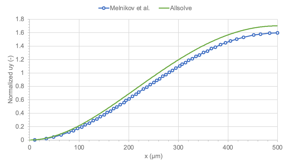
Fig. 10: Comparison of spatial displacement field (reconstructed from the harmonic data) at the center of the beam.
Simultaneous sweep over frequency and voltage
- 75 simulations - Freq: 20Hz-20kHz - Voltage: 5-25V - DoFs: 416k - 12 min run - 8 cores each
- Fig. 11 shows the total harmonic distortion as a function of driving frequency and voltage. The total harmonic distortion is often used to quantify the quality of sound signal output. With a harmonic balance approach, it is straightforward to perform sweeps over different parameters of interest, and explore the design space to find an optimal design.
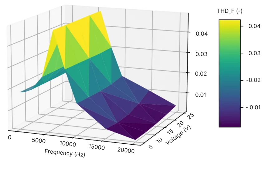
Fig. 11: The total harmonic distortion as a function of driving frequency and voltage.
Key benefits demonstrated
- Harmonic balance method was applied to a fully coupled multiphysics (electrostatics + solid mechanics + fluid dynamics) application including mesh deformation, geometric nonlinearity, and prestress.
- Nonlinear behavior was evidently captured and validated with the literature data.
- Frequency and voltage sweeps provide insights on the effects on output of interest in a given design space, which can be very useful in choosing an optimal design.
- Computational benefits were demonstrated in running parallel sweeps.
Other benefits of Quanscient Allsolve related to this topic
Quanscient Allsolve enables engineers to apply the harmonic balance method to a wide variety of problems, from small-scale electronics to large structural components. Its ability to handle complex physics, large models, and detailed interactions makes it a powerful tool for solving nonlinear problems. By combining this with cloud computing, Allsolve ensures that even resource-intensive simulations can be completed quickly and accurately.
Conclusion
Nonlinear systems are an essential part of engineering, and understanding their behavior is critical for designing efficient, reliable solutions. The harmonic balance method provides a practical and efficient way to study these systems, capturing their full range of behaviors in the frequency domain.
Quanscient Allsolve makes this method accessible for detailed and complex models by addressing the computational challenges through cloud-based resources. From Joule heating to beam vibrations and advanced microspeaker designs, the examples show how this approach delivers better results in less time and in the form of required engineering output parameters. As engineering challenges grow, tools like Allsolve will play an increasingly important role in creating innovative and effective solutions.
References
[1] Halbach A.: "Domain decomposition techniques for the nonlinear, steady-state, finite element simulation of MEMS ultrasonic", PhD Thesis, University of Liège, 2017.
[2] Nakhla M. S. and Vlach J.: "A piecewise harmonic balance technique for determination of the periodic response of nonlinear systems", IEEE Transactions on Circuits and Systems, vol. 23, pp. 85-91, 1976.
[5] Hayashi, S., Gutschmidt, S., Murray, R. et al. Experimental bifurcation analysis of a clamped beam with designed mechanical nonlinearity. Nonlinear Dyn 112, 15701–15717 (2024). https://doi.org/10.1007/s11071-024-09873-5
[7] Dr. Andrew Tweedie, Dr. Abhishek Deshmukh, Jukka Knuutinen. Faster and more reliable MEMS design with cloud-based multiphysics simulations. Quanscient webinars (2024). https://quanscient.com/events/mems-webinar-06-24/register
[8] Kaiser, B. et al. Concept and proof for an all-silicon MEMS micro speaker utilizing air chambers. Microsyst Nanoeng 5, 43 (2019). https://doi.org/10.1038/s41378-019-0095-9.
[9] Melnikov, A., Schenk, H.A.G., Monsalve, J.M. et al. Coulomb-actuated microbeams revisited: experimental and numerical modal decomposition of the saddle-node bifurcation. Microsyst Nanoeng 7, 41 (2021). https://doi.org/10.1038/s41378-021-00265-y.